📓 Depth and Breadth Search Algorithms

There are two ways we can search a tree — regardless of whether that's a binary search tree or a more general tree. We can take a depth-first search (DFS) approach or a breadth-first search (BFS) approach. You can probably guess a little bit about each approach. If we are looking at a tree that has a root node and child nodes, a depth-first search algorithm will search a tree vertically while a breadth-first search algorithm will search a tree horizontally. A graph can't really be measured vertically or horizontally in this way but the same concept still applies — we can search broadly or go deeper into each branch first. We just don't necessarily do so from a root node. Instead, we can start our search from any node in the graph.

Depth-First Search

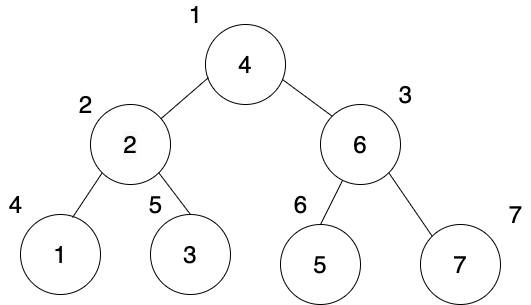
Remember our binary search tree application where we worked with a perfect binary search tree? If we wanted to do a depth-first search, we'd do so in this order.

We can say that the tree in this picture has four branches. They all start at the root node and terminate in a leaf node. So the left-most branch terminates at 1, the next branch terminates at 3, the next terminates at 5, and the last branch terminates at 7.

In a depth-first search, our algorithm will completely traverse the left-most branch. Once that is complete, it will backtrack (in this case, to the 2 node) and then completely traverse the next branch. It will continue doing this until it finds what it's searching for — or, if the value doesn't exist, until the tree is completely traversed.

But how does the algorithm actually backtrack? Well, a DFS algorithm commonly uses a stack (last-in, first-out) to search through each branch to the very end. Remember, to visualize a stack we can think of a stack of pancakes. The last pancake we add to a stack goes on top (the beginning of the stack) — and the first pancake we eat is the one on top — the last pancake on the stack is the first one we eat.

Let's walk through this process for our perfect binary search tree — and in doing so, we'll see how using a stack allows our algorithm to traverse and automatically backtrack through a tree's branches.

We'll start with the simple example — the one above — and then move onto a more complex example using a graph.

In the perfect binary search tree above, we start with the root node. Here's our stack so far:

let stack = [4]

There's only one element, so we can't really demonstrate its LIFO yet. We get the children of 4 (2 and 6) and remove the 4 from the stack. Now our stack looks like this:

stack = [2, 6];

Remember, we want to search the left-most branch first. So now we grab 2 from the beginning of the stack and add this node's children to the beginning of the stack: 1 and 3. Here's the stack now:

stack = [1, 3, 6];

Once again, to continue down the left-most branch, we just need to grab the first value. We take the 1 from the beginning of the stack. It has no children, so we are done with that branch. So here's our stack now:

stack = [3, 6];

Look at that — the first element in our stack is the next branch! We see that the 3 has no children of its own — so now our stack is just this:

stack = [6];

We've completely evaluated the left subtree and now only the right subtree remains. We take 6 from the stack, evaluate its children, and so on.

Now that we've looked at a basic example of how a DFS uses a stack, let's apply a more complex example. This time we'll use a graph. After all, we are in the middle of learning about graph theory.

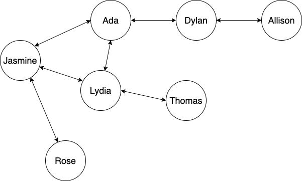
Here's a graph of friends. We will actually be using this very graph when we actually write our BFS and DFS algorithms over the next several lessons. Let's say we want to find a connection between Jasmine and Thomas. How would we do that with a depth-first search?

First, we'll get an array of Jasmine's friends. This is our initial stack:

let stack = ["Ada", "Lydia", "Rose"];

Now we want to navigate down through the first branch on the list. There's really no working from left-to-right here — nor can we really say we are searching the graph horizontally or vertically like we would with a binary search tree. Instead, we'd just grab the list of Jasmine's friends from an adjacency list or similar structure. Because this is a stack, we are starting with the first friend in the array. We remove Ada from the stack and get her list of friends.

Ada is connected to Dylan and Lydia. Let's add them to the top of the stack. Now our stack looks like this:

stack = ["Dylan", "Lydia", "Lydia", "Rose"];

Ada has been removed from the top of the stack while her friends have been added. Because this is a stack, we need to continue with the last-in, first-out approach. But now hopefully it's clear why we need to do that. What gets added to the top of the stack is any remaining friends in the branch we are currently traversing — as well as friends in sub-branches we will be traversing soon. Meanwhile, what's at the bottom of the stack? A completely different branch. So everything we add right now is what we need to evaluate right now — in other words, last-in, first-out.

So now we take Dylan from the top of the stack and grab his friends. There is just Allison, which we add to the top of the stack.

stack = ["Allison", "Lydia", "Lydia", "Rose"];

When we take Allison from the top of the stack, we'll see that she only has Dylan as a friend. However, we have already traversed the node that represents Dylan — and we don't want to traverse it again. To avoid that, we flag nodes as we traverse them. This is a key difference between how we'd traverse this graph versus how we'd traverse a binary search tree. Our binary search tree is directed — information can only flow from parents to children — and children know nothing about their parents. There is no risk of accidentally going back to a node that has already been traversed. However, our graph is undirected — so we need to make sure our algorithm doesn't accidentally traverse nodes that have already been covered.

So at this point, because we've traversed through nodes representing Jasmine, Ada and Dylan already, we wouldn't add them back to the stack. So when Allison is removed from the top of the stack, no one else is added.

So now our stack looks like this:

stack = ["Lydia", "Lydia", "Rose"];

We are moving onto our next branch! Once we reach the end of a branch, there are no more nodes to traverse. The last item in the stack will now be the most recent sub-branch we haven't explored yet. In this case, it is Lydia. But note that we are exploring Lydia's connection to Ada, not Lydia's connection to Jasmine here.

We remove that from the top of the stack and find Thomas. We've successfully determined the reachability between Thomas and Jasmine. So at this point, if we've been tracking our traversal, we can see that there's a connection going like this: Jasmine -> Ada -> Lydia -> Thomas. So we could say that Thomas is a friend of a friend of a friend.

But if we actually look at our graph, we can quickly see that there is a closer connection. After all, we normally call them friends of friends if we can — not friends of friends of friends. If we wanted to determine not just the reachability of a node but the shortest path, our depth-first search would continue.

By the way, here's a very important reason we need to flag nodes as we traverse them. Jasmine is Lydia's friend. If we didn't flag that we'd already traversed through that node, our algorithm could check Jasmine's friends, find Ada, and then check Ada's friends, find Lydia, and then check Lydia's friends, only to find Jasmine, forever and ever in an infinite loop of friends that sounds wonderful in practice but not in programming.

So the key takeaways here, at least from a programming perspective, is that we need to use a stack to walk through the graph with a depth-first search, and also that we need to flag nodes we've already traversed so we don't run into infinite loops or other inefficiencies.

If this is still confusing, don't worry. It should become clearer when we use TDD to write a depth-first search algorithm in the next lesson.

Advantages

• DFSs are great for building games because they allow the algorithm to explore winning and losing possibilities.
• If we know that the answer we are looking for will be at the bottom of a tree, a DFS will usually be faster than a BFS. For instance, we might be looking for living descendants of a long family tree — and everyone alive will be at the bottom of the tree.
• DFS usually takes less memory than BFS.

Breadth-First Search

On the other hand, a breadth-first search algorithm searches horizontally. The image below demonstrates this:

As we can see, the algorithm will search each row in the tree completely before moving onto the next one.

In contrast to a depth-first search, a breadth-first search uses a queue instead of a stack. That means that when we add new nodes to the collection, they are added at the end. Meanwhile, we evaluate the node at the beginning of the collection first. In other words, we're saying, hey, node, get in line! We'll get to you once we've gotten through all the nodes ahead of you.

Once again, let's demonstrate how this works first on the perfect binary search tree in the diagram above and then on our graph of friends.

Our queue starts like this:

let queue = [4];

We grab 4 and then add 2 and 6 to the queue.

queue = [2, 6];

2 is first in line, so let's add its children: 1 and 3. Here's the big difference between the stack we used before and the queue we are using now. We add 1 and 3 to the end of the queue — not to the beginning (or "top") of the stack.

So now our queue looks like this:

queue = [6, 1, 3];

We take 6 from the front and add its children (5 and 7) to the queue:

queue = [1, 3, 5, 7];

As we can see, we've finished an entire "row" of the tree — and all that's left to traverse is the bottom row.

Now let's look at the more complex example. Our graph of friends. Here's the picture of the graph again:

In this case, we want to check all of Jasmine's friends before we check her friends' friends.

First, we add all of her friends to an array:

let queue = ["Ada", "Lydia", "Rose"];

The first friend in the queue is Ada. We remove Ada from the queue and get her friends: Dylan and Lydia. We add them to the end of the queue:

queue = ["Lydia", "Rose", "Dylan", "Lydia"];

As we can see, the first few names still on the list are the ones that are Jasmine's friends — we save the names we added (friends of friends) to the end of the list. Remember, nodes added to the end of the list always represent going deeper into the tree. If we want to go depth-first, we add elements to the beginning of the collection. If we want to go breadth-first, we add new elements to the end of the collection.

If this is still confusing, we'll be covering BFS more in-depth — or maybe we should say more broadly — in the lesson after next.

Advantages

• If we know that an answer will be close to the root node, a BFS is more efficient. For instance, in the family tree example, we might be looking for a direct descendant that lived 50 years later than the ancestor at the root node, not 300 years later.
• BFSs are great for computing the most efficient path between two nodes. For that reason, they are great for GPS and mapping applications and even for finding people near each other in social networks.

Summary

In this lesson, we gave a brief overview of BFS and DFS algorithms, including the advantages of both. We also learned how depth-first algorithms utilize a stack (LIFO) while breadth-first algorithms use a queue (FIFO). At this point, we are ready to actually incorporate these algorithms into our graph application!